Category Archives: science

Genomic Imprinting III: The Loudest Voice Prevails

So, it’s been a while since the last installment of the Primers on Imprinting feature, but they should be posted with greater regularity in the upcoming weeks. This time we’re going to introduce something that we will see again in future installments: small differences in selection lead to large differences in behavior.

Last time, we introduced the most widely discussed and most successful explanation of the evolutionary origins of genomic imprinting, the “kinship” or “conflict” theory. According to this theory, imprinted gene expression is a consequence of the fact that natural selection acts differently on alleles depending on their parent of origin. There are several ways to think about the origin of this differential selection, but we talked about it in terms of the framework that I find most intuitive: inclusive fitness.

As we also noted last time, even in the cases where the asymmetry in selection on maternally and paternally derived alleles is sufficiently large to drive the evolution of imprinted gene expression, the actual magnitude of this asymmetry is actually incredibly small. Why? Well, even for a allele with large effects on the survival and reproduction of related individuals, the dominant factor in the inclusive fitness of that allele is still going to be the survival and reproduction of the individual organism carrying that allele around.

But, the standard pattern observed with imprinted genes is that the allele-specific expression is all or nothing. For example, an allele might be expressed when it is inherited from a male, but completely silent when inherited from a female. So this small difference in the optimal expression levels of the maternally and paternally derived alleles leads to – in a way – the largest possible difference in the realized expression levels of the two alleles.

I like to think of this in terms of an analogy. Imagine that Pat and Chris share an office, and that they have a slight disagreement over the temperature they want the office at. Say Pat wants the office to be at 71 degrees (Fahrenheit), while Chris wants it to be 70. Each of them has control over a small space heater, and this is the only mechanism that they have for manipulating the temperature. [1]

What’s going to happen? Let’s say the temperature is 70 degrees. Pat will turn up his/her space heater until the temperature reaches 71. In response, Chris will turn his/her space heater down until the temperature comes down to 70. They will go back and forth like this until, eventually, Chris’s space heater is completely turned off. Pat will then turn his/her space heater up to get the room to 71. Then we’re done. Chris is unhappy about the temperature of the room, but no longer has any ability to make it any cooler.

Two things about this outcome. First, a small disagreement over the ideal temperature has led to a large divergence in the strategies: Chris’s space heater is all the way off, while Pat’s is on and doing all the work. Notice that the outcome would be exactly the same, in principle, if Chris’s ideal temperature were 70.9 degrees, or even 70.999 degrees. [2]

Second, Pat wins. This is a consequence of the fact that we are talking about space heaters, and that Pat prefers the higher temperature. If, instead of space heaters, Pat and Chris each had control of an air conditioner, Chris would be the winner. At equilibrium, Pat’s air conditioner would be all the way off, and the room would be at 70 degrees.

This is also the way it works with alleles at an imprinted locus. Let’s consider the case of a gene where increased expression results in increased prenatal growth. The inclusive fitness argument says that the optimal amount of this growth factor is higher for an allele when it is paternally inherited than when it is maternally inherited. Say this patrilineal optimum is 105 units, while the maternal optimum is 95 units.

If the gene is not imprinted we might expect it to produce about 100 units, with each allele producing 50. However, once the evolutionary dynamics of imprinting take over, the pattern of expression will evolve to one where alleles are transcriptionally silent when maternally inherited, but where a paternally expressed allele is making 105 units.

For a growth-suppressing gene, where increased expression actually reduces prenatal growth, we expect the opposite pattern, where alleles are silenced when paternally inherited, but are expressed when maternally inherited. This set of predictions – that imprinted growth enhancers will be paternally expressed, and imprinted growth suppressors will be maternally expressed – matches the empirically observed pattern by and large, although there are a few counterexamples that are not fully understood at the moment.

This pattern of allele silencing has been dubbed the “loudest voice prevails” principle. The phenotype evolves to the optimum of the allele favoring higher expression. Now, you can argue that this is the sort of thing that does not really need its own name. Fair enough. It’s really just saying that the evolutionarily stable state of the system is an edge solution. But, “loudest voice prevails” is sort of catchy, and has the advantage of reminding us which allele is expressed at equilibrium.

The Haig 1996 citation is the paper that introduces the phrase. The other three citations are papers published around the same time that use different mathematical frameworks to address the evolution of gene expression at an imprinted locus. Generically speaking, the answer is the one described here, although the Spencer, Feldman, and Clark paper identifies certain regimes in parameter space where apparently different results can be obtained. In a future post, we will delve into the differences in the assumptions and conclusions of different modeling frameworks as they have been applied to imprinting.

Now, what if you consider more than one imprinted gene? What if Pat and Chris each have a space heater and an air conditioner? We’ll talk about that next time.

Haig, D. (1996). Placental hormones, genomic imprinting, and maternal-fetal communication Journal of Evolutionary Biology, 9 (3), 357-380 DOI: 10.1046/j.1420-9101.1996.9030357.x

Mochizuki A, Takeda Y, & Iwasa Y (1996). The evolution of genomic imprinting. Genetics, 144 (3), 1283-95 PMID: 8913768

Haig, D. (1997). Parental antagonism, relatedness asymmetries, and genomic imprinting Proceedings of the Royal Society B: Biological Sciences, 264 (1388), 1657-1662 DOI: 10.1098/rspb.1997.0230

Spencer HG, Feldman MW, & Clark AG (1998). Genetic conflicts, multiple paternity and the evolution of genomic imprinting. Genetics, 148 (2), 893-904 PMID: 9504935

–––––––––––––––––––––––––––––––––––––––

[1] Of course, in the real-life situation, we might assume that Pat and Chris would discuss the situation and come to some sort of agreement. This is a key difference between people interacting in strategic situations and genes evolving under natural selection. Alleles at a locus are like people sharing an office, where both of them are incredibly passive aggressive. If it helps, imagine that Pat and Chris won’t talk to each other.

[2] In practice, of course, there is going to be some minimum level of disagreement required in order to trigger this passive-aggressive escalation. In this analogy, the minimum level will be set by a combination of things such as the sensitivity of Pat and Chris to small changes in temperature, the precision with which the space heaters control the temperature of the room, and the extent to which they care about each other’s comfort. Similar reasoning holds in the case of genes, and we will address this in a future installment of the series, where we ask why there are any genes that are not imprinted.
Google Violates Benford’s Law, Arrest Warrant Issued

So, Google has already had it’s Twitter account subpoenaed, and can look forward to months of molestation enhanced screening at the airport, all thanks to its brazen violation of Benford’s Law.

What is this Benford’s Law thing?

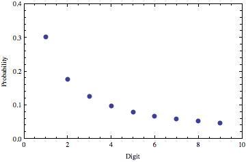
It is a statement that if you look at lists of numbers in empirical data, the first non-zero digit is distributed in a very specific way. At least for certain kinds of data. Specifically, if the logarithms of the numbers you are looking at are uniformly distributed, then the first digits of those numbers will be Benfordly distributed.

Here’s what the relative probabilities of different first digits look like:

Here’s a graphic that shows the frequencies of different letters and numbers in Google searches. The numbers are way down at the bottom.

Image via Gizmodo

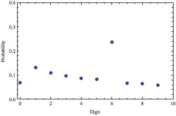
The thing that you’ll notice about this is that 6 is by far the most common digit (and that J/j is sad). Here’s a plot of these relative frequencies on the same scale as the Benford’s Law plot above.

Roughly speaking, this plot has the same shape as the one above, except for the fact that it includes 0, and that 6 is crazy. But, look at where the 0 value is: pretty much even with where you might expect the 6 to be. What happens if we assume that this was actually a transcription error that happened somewhere along the way? If we switch the 6 and 0 values, and then look at the relative probabilities of all of the non-zero digits, we get this:

The dark blue dots are the Benford’s Law points that we showed before. The reddish squares are the new empirical distribution.

Now that we’ve switched the 6 and the 0, we get something that looks to me like a mixture of the Benford’s Law distribution and a uniform distribution. But remember, Benford’s Law applies to first digits. This is data from all google searches. So, that’s going to be a mixture of first digits and non-first digits.

If we assume that 35% of the non-zero digits in searches are first digits, and that the other 65% are uniformly distributed between 1 and 9, we can back out the relative frequencies of the digits specifically in the first digit context.

The blue circles are the Benford’s Law expectations, and the red squares are the inferred empirical distribution of first digits. The choice of 35% was established through manual trial and error, and the fit was done by visual inspection. So, you know, don’t go and make any medical decisions based on this.

This is actually a reasonably good fit for this sort of thing, and constitutes fairly compelling evidence in support of the “sumbudy dun messed up” theory to my mind. Either that, or you have to invoke roughly 6 billion instances of people googling ‘666’.

Frank Benford (1938). The law of anomalous numbers Proceedings of the American Philosophical Society, 78 (4), 551-572

The Genetical Book Review: Middlesex

So, welcome to the first installment of Lost in Transcription’s newest feature: The Genetical Book Review. For the maiden voyage, we’ll cover the 2002, Pulitzer-prize-winning Middlesex by Jeffrey Eugenides.

You’re surprised? Because you assume that an eight-year-old Pulitzer winner must already have been reviewed?

Fair enough. But, here’s the gimmick: we’ll use the genetics angle to talk about some things that have not already been covered extensively elsewhere.

First, though, the precis and value judgement. If you’ve not read the book, or read about it, it follows three generations of the Greek-American Stephanides family, who traipse through a slice of historical events in Smyrna and Detroit over the course of nearly a century. It’s sort of a Forrest Gump for the NPR set. Cal Stephanides and his relatives witness genocide at the hands of the Turks, emigrate to America, build cars for Henry Ford, and run booze during prohibition. They are present for the founding of the Nation of Islam and the 1967 Detroit race riots. They flee to the suburbs and watch Watergate unfold on the television.

As in Forrest Gump, some of the historical context feels a bit like pandering, an attempt to draw the reader in through nostalgia. On the other hand, many of the events are local enough to be only passingly familiar to most readers, so there’s learning to be had. More importantly, those events are always portrayed through the lens of how they shaped the trajectories of the characters in the book. And, they are charmingly and engagingly written, with a varied style that is pleasurable to read.

Basically, if your book group has not already read this book, and you’re sick of plodding stories about alcoholic mothers and victims of sexual abuse, but want something with some literary gravitas (so that you don’t lose social status by suggesting it to your book-group frenemies), this is the book for you!

There you have it. Hit the jump for the role of genetics in the book.

The book is written in a memoir style, told by Cal, who periodically takes on the persona of a chromosome being passed down, or an egg sitting in an ovary as s/he relates the events from previous generations. I say “s/he” because – and I’m not giving anything away here – the key twist to the coming-of-age story is that Cal is intersex, having ambiguous genitals as a result of a recessive, genetic 5-alpha-reductase deficiency.  For reasons reaching back to Smyrna, Cal’s condition is not identified at birth, and our protagonist is raised as a female, Calliope. It is not until puberty hits that Calliope discovers her condition and transforms into her male alter ego, Cal.

The 5-alpha-reductase gene encodes an enzyme that converts testosterone into dihydrotestosterone (DHT). In early development, testosterone is responsible for certain internal male reproductive structures, such as the vas deferens, while DHT is responsible for the external genitalia. Upon the onset of puberty, testosterone drives the male increase in muscle mass and deepening of voice, while DHT is responsible for the growth of facial hair. One of the reasons for the female-to-male switch that happens at puberty is that there are actually two different 5-alpha reductases. The type 2 enzyme is the one that is primarily responsible for DHT production, particularly in early development, and it is this enzyme that Cal lacks. The other one, the type 1 enzyme, is substantially upregulated at puberty, which results in an uptick in DHT production.

So, there are two things that combine at puberty to drive the sudden appearance of male characteristics: (1) Testosterone and DHT start sharing the load for creating external male-typical characteristics, and (2) a second pathway appears for the generation of DHT.

I have to say, as I have read about this disorder, I have been impressed with the depth of understanding that Eugenides seems to have brought to the novel.

[As a side note, this disorder was first identified in the remote village of Salinas in the Dominican Republic, where it occurred in about 2% of live births. Locally, these individuals are known as “guevedoces.” Whenever I have seen reference to the guevedoces, it is followed by the phrase “literally ‘penis at twelve.'” Actually, it turns out that ‘gueve’ is derived from ‘huevos,’ which is slang for ‘balls.’ Thus, a better translation might be “balls at twelve.” Although, if you’re going to precede your translation with “literally,” you would need to acknowledge that this slang for ‘balls’ is literally the word for ‘eggs.’ Of course, referring to the appearance of male sexual characteristics at the onset of puberty as “eggs at twelve” is just weird and confusing, because it sounds like something you would order at Denny’s, and because it is sort of the exact opposite of what is going on.]

Incest is one of the recurring themes in the book, which traces the paths through which Cal came to inherit two defective copies of the 5-alpha-reductase gene. This particular disorder is straight-up recessive, so if you have one functional copy of the gene, you develop normally.

Cal’s grandparents on his/her father’s side are brother and sister. They hailed from the same tiny village outside of Smyrna, were orphaned, and fell in love. Their immigration to America permitted them the opportunity to fabricate a non-consanguinous past. The interesting thing is that the inbreeding involving Cal’s grandparents bears absolutely no responsibility for Cal’s condition. Their son, Milt is unaffected, which means that he inherited one defective gene copy from one of his parents. It doesn’t actually matter whether the other parent carried a copy or not.
More specifically, what is required for the story is that Milt be a carrier, but not express the condition. If one of his parents is a carrier, the probability that he is a non-expressing carrier is 1/2. If both of his parents are carriers, the probability that he is a non-expressing carrier is 1/2. It will not have escaped your attention that 1/2 = 1/2.

There is a second case of inbreeding, however, that does contribute to Cal’s condition. Milt and his wife, Tessie, are second cousins, and each of them is heterozygous for the deficiency. Now, statistically speaking, the fact that Milt and Tessie are second cousins barely counts as incest. For a rare disorder such as 5-alpha-reductase deficiency, the elevation in risk due to a second-cousin marriage is small. How small? Let’s see.

Assume that the frequency of the defective version of the gene is q = 0.001, or one in a thousand. This is in the ballpark of what we might expect for a recessive mutation maintained at mutation-selection balance. The probability that an outbred individual inherits two defective copies is approximately q2, or one in a million. What if the mother and father are related? If their degree of relatedness is r, then the probability that their child will inherit two copies is:

         p = q (r/2q (1 – r/2))

What is this r thing? Well, if they are brother and sister, r = 1/2, so the probability p would be about 0.00025. For first cousins, r = 1/8, and p = 0.0000634. For second cousins, r = 1/32, and p = 0.0000166.

That is, for second cousins, the probability goes from one in a million to about one in 60,000. Basically, you will have a bigger impact by taking prenatal vitamins.

Diane Paul and Hamish Spencer published an interesting piece a couple of years ago about the history of the stigmatization of first-cousin marriage, particularly in the United States. They make a number of interesting points, and I recommend the article, which can be found here. It is short, fascinating, open access, and requires no background in genetics to follow.

One of the points they make is that there is pretty much no way to interpret a ban on first-cousin marriage as anything other than eugenics. And yet, somehow, this prohibition has managed to escape that label. Another of their points is that the genetic risks associated with first-cousin marriage are actually small compared with a lot of behaviors that are completely acceptable in our society, such as women having children over the age of 40, or the use of in vitro fertilization techniques. (That second one was not mentioned by them, but it’s true.) So, there is some inconsistency there, which they trace to nineteenth century misconceptions about heredity and prejudice against immigrants and the rural poor.

But, back to the book.

To recap, in terms of causal things leading to Cal’s genetic composition, the fact that his/her parents are second cousins matters. The fact that the grandparents are brother and sister does not. Why, then, does the story, much of which is driving towards Cal’s conception, spend so much more attention on the (genetically) irrelevant grandparental love story?

Obviously, I can’t speak to the author’s intention, but to me, having two separate incidents provides a nice, clean separation between the psychological and genetic consequences of incest. Cal’s grandmother is wracked with guilt about her transgression, and this guilt drives the story in several places. In fact, one of the motifs in the book is that action (or, often, lack of action) is often motivated by superstitious beliefs. –– Sorry about the vagueness here. I’m in spoiler-avoidance mode. –– Hypothetically speaking, let’s say one of the characters is eating toast, and then that character’s mother falls down and breaks her hip. The character would blame him/herself for eating toast and refuse to eat toast again for a long time. You get the idea.

Anyway, my point is that by having two separate incests, we are able to distinguish more clearly between the genetic consequences of consanguinity from the EWWWW consequences of knocking boots with your sister.

Paul, D., & Spencer, H. (2008). “It’s Ok, We’re Not Cousins by Blood”: The Cousin Marriage Controversy in Historical Perspective PLoS Biology, 6 (12) DOI: 10.1371/journal.pbio.0060320

Buy it now!!

What’s that? You say you want to buy this book? And you want to support Lost in Transcription at the same time? Well, for you, sir and/or madam, I present these links.

Buy Middlesex now through:

Amazon

Barnes and Nobleicon

indiebound

Alibrisicon

The Cost of Christmas

So, if you haven’t already, you’ll probably soon receive the credit card bill with all of your Christmas purchases on it. Was it worth it? Well, was it, punk?

If you’re like most people, some of your presents were probably intended to impress someone. The question is, what’s the best kind of present for that? Should I give the girl from math class diamond earrings, or new batteries for her calculator? Should I give my boss a mug, or a gift certificate to Glamour Shots?

Fortunately, Science!™ has the answer. Today’s journal club entry concerns a model of gift-giving that considers three different types of gift that differ in their cost to the giver and their value to the recipient. “Cheap” gifts are, well, cheap. “Valuable” gifts are expensive to give, and have value to the recipient. The interesting category is the third one, the “extravagant” gifts, which are expensive to give, but have little inherent value to the recipient.

The specific context is gift-giving and mating. The model is of a sequential game with three or four stages. First, the male offers a gift to the female. Second, the female either accepts or rejects the gift. Third, she chooses whether or not to mate with the male. Then, in one version of the game, the male decides whether or not to stick around and contribute to the care of the offspring.

This $305 luxury frisbee is an example of an extravagant gift.

The conclusion of the paper is that there are many combinations of parameter values that will lead to males giving extravagant gifts. There are two critical features of the model that seem to be necessary in order to get this result.

First, there is uncertainty. The female has a guess about the quality of the male (or, equivalently, in the version of the model with paternal care, the probability that he will stick around after mating). By accepting the gift, she gains additional information about his quality or intentions. Similarly, the male is uncertain about the quality and intentions of the female – whether it is worth it for him to stick around after mating, and whether or not she is a gold-digger, who will just take his gift and skip town with his cousin.

[Editorial note: the term “gold-digger” is from the paper. Those of you who know me know me know that I would never have gone with such a politically incorrect term. I would have used “■■■■■■■■■■”.]

[[Meta-editorial note: parts of the previous editorial note have been redacted.]]

The other key feature is that there must be some cost to the female in accepting the gift.

Now, there are lots of parameters in a model like this, and several equilibrium solutions are possible. The interesting one is the one where males give cheap gifts to unattractive females (females whom they judge, with some uncertainty, to be of low quality), and give extravagant gifts to attractive females.

The key to getting the interesting equilibrium is that the ability or willingness to provide and extravagant gift has to correlate with the male’s quality or intentions. For example, a male can’t afford to spend two-months salary on a diamond ring every time he wants to have a one-night stand. Therefore, an extravagant engagement ring becomes a reliable indicator of his intentions. Ideally, the gift has to have no inherent value to the female, for example, if it were impossible to sell the engagement ring for cash money. Recall also that it has to cost her something to accept the gift. Then, taking the gift constitutes a commitment on her part as well. Otherwise, she benefits most from accepting the gift and walking away.

In the salacious application-to-human-mating case, this cost to the female is easiest to envision as a reputation cost (e.g., the risk of being labeled as a ■■■■■■■■■■). In certain species, where females mate with multiple males, store the sperm, and then use it selectively, there may be direct opportunity costs that do not require catty moralizing.

Just one last point.

The paper starts with, “Gift-giving is a feature of human courtship”. The authors cite Geoffrey Miller’s 2000 book, The Mating Mind. If the paper were being written today, I assume they would have cited more recent work by Hefner and Harris.

Sozou, P., & Seymour, R. (2005). Costly but worthless gifts facilitate courtship Proceedings of the Royal Society B: Biological Sciences, 272 (1575), 1877-1884 DOI: 10.1098/rspb.2005.3152

State-by-State FST(ish) Values: The Structure of Racial Diversity in America

So, in the world of population genetics, as in the real world, people are often interested in diversity, and in how that diversity is distributed. In biological contexts, quantifying these things is important because it gives us insight into the processes – like reproduction, migration, selection, etc. – responsible for generating the observed patterns of diversity.

Here I look at how racial diversity is apportioned among counties (or county equivalents) in each of the 50 states, using two different statistics derived from the population genetics and ecology literature. Hit the jump for the analysis, and scroll down to skip the introduction and go straight to the maps.


One of the earliest and most enduring quantities in population genetics is FST. This quantity (along with various closely related “F”s with different subscripts) is an attempt to create a metric of population differentiation that is independent of the overall level of diversity. There are a variety of ways of formulating FST, depending on the type of data you’re thinking about, but all are something like this:

FST = (Db – Dw) / Db

Here, FST is a measure of differentiation between or among subpopulations. Dw is the diversity within subpopulations, and Db is the diversity among subpopulations. As you can see, if you simply double the level of diversity (both within and among subpopulations), this measure of differentiation will be unchanged.

The concept of FST was developed 80-90 years ago, primarily by Sewall Wright, who examined and characterized some of its properties within highly simplified and idealized models of population structure. Then, 40-50 years ago, people started thinking about ways to estimate this quantity from genetic data. A lot of FST-related statistics have been developed, but I will described just one here, which compares the observed and expected levels of heterozygosity:

GST = 1 – HO/HE

HE is the observed level of heterozygosity. Roughly speaking, we look at some gene all of the individuals in the population. Each person has two copies of the gene. If the two copies are the identical, the person is homozygous; if they are different, the person is heterozygous. The observed heterozygosity simply the fraction of people who carry two different copies.

The expected heterozygosity, HE is calculated by taking all of the genes in the population and mixing them together. Now, draw two gene copies at random and ask, what is the probability that the two gene copies are different?

If the population is completely well mixed, HO and HE will be nearly the same, and GST will be close to zero. Elevated levels of GST result from non-random mating. For example, if the population consists of two isolated subpopulations, those subpopulations will tend to contain different versions of the gene, but there will be no one who has one copy of a variant from subpopulation 1 and a variant from subpopulation 2. Thus, there will be a reduced number of heterozygotes in the population, relative to what you would get if you mixed all of the genes in the two subpopulations together.

This notion of heterozygosity is not limited to genetic contexts, however, and we can do the equivalent calculation for any trait that can be divided into distinct categories (even if those categories are somewhat arbitrary social constructs like “race”).

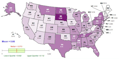
Here’s an illustration. I have taken data from the 2009 American Community Survey, aggregated at the level of individual counties. I calculate the “observed heterozygosity” from the frequencies of different races in each county. Imagine that within each county, we paired people at random. The HO calculated here is the fraction of these randomly paired couples who would have mixed-race children. In this calculation, I have assumed that if one parent self-identifies as “two or more races,” the children are mixed race, independent of the race of the other parent. Also, for simplicity, I have aggregated all subdivisions of “hispanic” into a single category. The HE here is calculated from the same random-mating procedure applied at the level of the entire state.

Here is a map of the results, generated using the free, online map generator from the National Council of Teachers of Mathematics:

Darker colors correspond to higher values of GST.

Now, it has been known for a long time that FST is not particularly well behaved. It is sensitive to things like the total number of distinct gene variants in the population and the total number of subpopulations. Recently, researchers have begun developing corrections to estimators of FST that are more robust to these deviations from the ideal models originally studied by Wright. One such correction was published a couple of years ago by Lou Jost, who proposed a metric, D, which demonstrably has many desirable properties that we would like to see from a statistic that describes population differentiation. In terms of the heterozygosities that go into GST, D is calculated like this:

D = [(HE-HO)/(1-HO)][n/(n-1)]

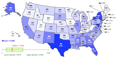
where n is the number of subpopulations. We can recalculate the racial “population differentiation” at the county level for each state. The new map looks like this:

As in the previous map, darker colors represent higher values of D.

Now, there are a lot of reasons to exercise caution in interpreting these values. The Jost correction used to generate the second corrects for certain problems associated with GST, but there is still an issue in that this analysis is based on aggregation at the county level. The geographical extent of counties varies enormously from state to state; the meaning of being in the same county in Utah is quite different from being in the same county in New York. Furthermore, the frequencies and identities of the groups vary among states in a way that will matter much more to any sociological analysis than will the numbers presented here. The FST-related statistics used here have been developed in the context of biological data, with the goal of understanding biological processes that are not necessarily analogous to the social processes that have driven the distribution of various groups in the US.

On the other hand, it is a lot more fun NOT to exercise caution. To that end, here is your list of the ten most racially differentiated states based on Jost’s D (second map):

Maryland, Texas, New York, Florida, Alaska, Mississippi, Georgia, New Mexico, New Jersey, California

And the ten least differentiated:

Vermont, Maine, New Hampshire, West Virginia, Iowa, Wyoming, Utah, Delaware, Minnesota, Idaho

If we go back to the raw GST (first map) the top-ten most differentiated are:

South Dakota, Maryland, North Dakota, Tennessee, New York, Montana, Texas, Pennsylvania, Florida, Alaska

And the least:

Vermont, Maine, Delaware, New Hampshire, Hawaii, West Virginia, Connecticut, Nevada, Utah, Oregon

I will leave irresponsible speculation and stereotyping of the residents of different states as an exercise for the reader.

JOST, L. (2008). GST and its relatives do not measure differentiation
Molecular Ecology, 17 (18), 4015-4026 DOI: 10.1111/j.1365-294X.2008.03887.x

Where stalkers become friends: Geo-tagging on Flickr

So, you probably remember this from the most recent episode of The Mentalist / Bones / Castle / Criminal Minds / Numb3rs:

SEXY YET PROFESSIONAL DETECTIVE: What have we got?

SASSY JUNIOR DETECTIVE: Nothing. All of our leads have dried up like Cher’s ovaries.

GRUFF SENIOR LAW ENFORCEMENT OFFICIAL: We’ve got to wrap this thing up. I’ve got the mayor breathing down my neck.

MAYOR: Hhhhhhhhhh. Hhhhhhhhhh.

G.S.L.E.O.: And now he’s drooling.

S.Y.P.D.: We’ll keep after it, but we’re a bit short-handed after half of the department was beheaded and, ironically, eaten by The Vegan Killer.

G.S.L.E.O.: I don’t want excuses. I want someone behind bars.

S.J.D.: You and my alcoholic ex wife.

SOCIALLY INAPPROPRIATE GENIUS: Actually, we know that the comptroller picked up his dry-cleaning on Wednesday. The same Wednesday that the chimney sweep showed up at the wedding in a curiously un-besooted pair of dungarees. Thus, the heiress was murdered by the delivery man who brought the Martinizing agents to the dry cleaners, also on Wednesday. Also, he was her half brother.

And, scene.

Thanks to research just published in PNAS by a group out of Cornell, we are now one step closer to living in a dystopian panopticon in which our associations can be inferred by any monkey with a laptop. Soon, Patrick Jane will be back to doing parlor tricks, Richard Castle will be back to making a living as an imaginary writer, and everyone else will be in prison for consorting with each other.
More specifically, the authors investigate whether they can infer a social connection between two people on the basis of their having been at the same place at the same time on multiple occasions, using data from Flickr. They look at 38 million pictures that contain both a timestamp and a geo-tag, indicating the time, latitude, and longitude at which the picture was taken. They define a co-occurrence of two Flickr users as having pictures taken within a time t of each other and within the same geographic region: a square(ish) region of length s latitude or longitude degrees on each side. The social dimension of the data comes from Flickr’s networking functions, which allow users to specify their links to others. 
They find that the greater the number of co-occurrences for a pair of users, the more likely it is that they are friends. This is not particularly surprising, although the magnitude of the effects are quite striking. For example, here is one graph from the paper:
Part of Figure 2D from the paper. In this case, the spatial range for co-occurrence is defined by s = 1.0 degrees (about 55 miles by 65 miles where I live). The different curves correspond to different time windows.

The probability that two randomly selected Flickr users are friends is less than 1 in 7000 [Corrected. Original post said 1 in 700]. However, if two users have uploaded pictures from the same 1 degree by 1 degree region within a day of each other on five different occasions, there is nearly a 60% chance that they are friends. If they have done it more than eight times, the chance is more than 90%.

In other words, if you and your accomplice both upload photos from the same dry cleaner every Wednesday, even a non-genius will be able to figure out that you know each other. This is how Strangers on a Train will end in the 2032 remake starring Freddie Highmore and Abigail Breslin.

For those interested in looking at more pretty graphs, the article is Open Access, and can be found here.

For those interested in mounting a futile defense against the Orwellian State, more information about geo-tagging and privacy can be found here, including ways in which you may inadvertently be sharing location information without meaning to.

Crandall, D., Backstrom, L., Cosley, D., Suri, S., Huttenlocher, D., & Kleinberg, J. (2010). Inferring social ties from geographic coincidences Proceedings of the National Academy of Sciences DOI: 10.1073/pnas.1006155107

The Distribution of Dominance

So, as you have no doubt surmised from the title of this post, the cash-strapped Republican Party is going to start using their abundant frequent “flyer” points to pay their debts.

I’m kidding, of course. The GOP doesn’t pay its debts!

Actually, we’re going to talk about a paper just out in Genetics by Aneil Agarwal and Michael Whitlock. They provide a very thorough analysis of data on the fitness effects of homozygous and heterozygous gene deletions in yeast.

But let’s back up for a minute first.

The authors are interested in understanding the distribution of dominance, in the population-genetic sense. Traditionally, the dominance is represented by h, and the strength of selection by s. Usually, we define the fitness of the wild-type (hypothetically not carrying any mutations) as 1. Then, we consider the fitness effect of a mutation in a particular gene. In this case, we’re going to focus on deleterious, or harmful mutations, which reduce fitness. If an individual carries two copies of the deleterious mutation, they have a fitness of 1-s, so that small values of s mean weak selection, and large values of s mean strong selection. The dominance refers to the relative fitness of an individual carrying only one copy of the deleterious mutation. This heterozygous fitness is 1-hs. If h equals 1, the deleterious mutation is completely dominant, meaning that having one copy of it is just as bad as having two. If h equals 0, the deleterious mutation is completely recessive, and having one defective copy of the gene is just as good as having two functional copies.

So, what is a typical value of h? Does it depend on s? How much does it vary from gene to gene? The conventional wisdom is that most deleterious mutations are recessive. This is why you should not have children with close relatives. I carry a bunch of recessive mutations, as does my wife. As long as we have different ones, our son inherits a bunch of mutations – but only one copy of each – so they’re recessive in him as well. If we were closely related, we would carry many of the same mutations, and there would be a decent chance that our son would inherit two defective copies of the same gene, which could have various health consequences.

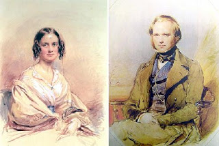
Charles Darwin and his first cousin Emma Wedgwood were married in 1839. 170 years later, they were portrayed by real-life-non-first-cousin couple Paul Bettany and Jennifer Connelly (not pictured).

However, population geneticists don’t care about things like this just because of the implications for human disease. Dominance has a major impact on the eventual fates of individual mutations, and can influence other evolutionary processes, like speciation. Often, in order to model some other process, we have to make some sort of assumption about the distribution of fitness effects of mutations. Traditionally, a researcher would pull this distribution out of his or her asc. This is one of the biggest contributions that this paper will make to the field. It provides a nice, empirically based distribution of dominance effects that can feed into other evolutionary studies.

The results also confirmed (with much greater confidence than was previously the case) the relationship between h and s which had been suggested by some previous studies. They find that larger values of s tend to go with smaller values of h. Consistent with the conventional wisdom about not marrying your cousin, strongly deleterious genes tend to be pretty recessive. More surprisingly, most mildly deleterious mutations had fairly high h values. In fact, the mean value of h over all deleterious mutations was 0.8 – quite dominant. However, when the average is weighted by the fitness effect s, it drops to 0.2.

The authors also point out that this negative relationship between h and s has implications for the evolution of dominance. This pattern is most consistent with theories in which dominance is shaped by indirect selection. For example, deleterious mutations might be recessive if the protein produced by the gene were selected for overexpression to enhance a metabolic pathway, or to buffer the performance of that pathway in certain environments. Then, loss of one copy of the gene encoding that protein might not have a major effect on function (half of too much being still enough). Alternatively, recessiveness could come from feedback mechanisms that upregulate the functional copy of the gene when not enough of the gene product is being made.

The point is that in either of these cases (among others), recessiveness is driven by selection to maintain the function of the gene. The more important the gene is (the larger the value of s associated with it), the stronger this selection will be, and the more recessive deleterious mutations will become. Therefore, mechanisms like these predict the observed negative relationship between h and s.

On a historical note, this type of buffering process was proposed by one of the giants of population genetics, J. B. S. Haldane way back in 1930. Haldane passed away on December 1, 1964.

R. I. P., J. B. S.

Agrawal, A., & Whitlock, M. (2010). Inferences About the Distribution of Dominance Drawn from Yeast Gene Knockout Data Genetics DOI: 10.1534/genetics.110.124560

Concerning a Way for the Prolongation of Humane Life

So, Deare Readers of this Blogue, I hope that you will indulge me in reporting on an Interesting Idea published by the Royal Society in their Philosophical Transactions. I hope, Deare Reader, that you may also see fit to join me in Lauding said Society for having made their entyre back catalogue freely available to the publick this Month of November.

The Publication in Question, titled An Extract of a Letter Written by Monsieur de Martel of Montauban to the Publisher, Concerning a Way for the Prolongation of Humane Life, together with Some Observations Made in the Southern Parts of France, English’d as Follows, contains the author’s reflections on the Causes of the Debilitation of Nature’s strength in the course of man’s life, and how these Causes might be Ameliorated, leading, naturally, to a means of achieving Eternal Youth through Medical Science.

The author agrees with the illustrious Messrs. Bacon and Sanctorius that the extinction of the natural heat and dessication of the Radical humour, as previously understood by Philosophers, seem not sufficient explanation for the causes of Age. However, Monsieur de Martel disagrees with Sanctorius’s assertion that “the Fibres do dry up, that they can no more be renew’d,” noting that even old Oxen have at certain times more or less marrow (though not, he is quick to point out, owing to the cycles of the moon).

Blood, claims Monsieur de Martel, is the Principle of Life, but notes that a Man typically has no Shortage of Blood when he dies. What causes this man to age, then, is that the Veins and Arteries which inclose the Blood, much like the Chymists Furnace, develop apertures, which, being insufficiently repair’d, do ease the dissipation of the igneous particles, such that they abandon the Blood. He reasons, then

 As in Stuffs and Cloth (whose woof is in manner like that of the Tunicles) the Threds by wearing do loosen and break, insomuch that many holes are made in it as in a Sieve. So that, if we had the Art to reinforce and to strengthen anew those Coats and Membranes, that they might not let slip what maketh the blood vital, the life would be preserved perpetually. . . . There is no reason to despair of finding out such Medicins, or Ailments, as are proper to strengthen the Coats and Membranes of the Vessels, so that they may at all times retain the fiery and spirituous corpuscules of the blood, as well as in the time of Youth.

The author also reports on the method of making Muscadin Wine in Frontignac.

For those wishing further to pursue Monsieur de Martel’s ideas on the Acquisition of Eternal Youth through preservation of the blood’s vital igneous particles, or those wishing to instruct their Slaves on how best to produce a nice Muscadin, the citation information is:

de Martel, M. (1670). An Extract of a Letter Written by Monsieur de Martel of Montauban to the Publisher, Concerning a Way for the Prolongation of Humane Life, together with Some Observations Made in the Southern Parts of France, English’d as Follows Philosophical Transactions of the Royal Society of London, 5 (57-68), 1179-1184 DOI: 10.1098/rstl.1670.0020

Irony Alert: Marc Hauser on moral judgments

So, PNAS has just published a brief exchange on the nature of moral judgments, including a letter where one of the coauthors is the man who put the a** in a**ertainment bias.

Marc Hauser is a Professor in the Psychology Department at Harvard. He made a name for himself publishing a variety of behavioral and cognitive studies on both humans and non-human primates, with the goal of understanding the evolutionary origins of human cognition, including complex traits such as language, economic decision-making, and moral judgments. More recently, he has made a name for himself by allegedly falsifying data and allegedly bullying the people in his lab who naively thought that the data published by the group should be . . . I don’t know . . . NOT falsified. I won’t repeat what this more recent name that he’s made for himself is, as it would violate the norms of internet civility. Over his career, Hauser has published something like 200 articles and 6 books, many of which probably contain certain things that are not entirely false. At the moment, he is on leave from Harvard, following an investigation’s finding him solely responsible for 8 counts of scientific misconduct. Presumably, he is working on his next book, allegedly titled Evilicious: Explaining Our Evolved Taste for Being Bad.

Snarking aside, the two letters that were just published follow from an interesting article published in PNAS earlier this year, where Hauser is the third of four co-authors. For those not familiar with authorship conventions in biology and related fields, here is what is typically implied by the order of authorship on a four-author paper. The first author probably did all of the experiments. The second author helped with some of the experiments, and/or some of the data analysis. The third author probably didn’t directly participate, but contributed ideas and/or reagents and/or equipment. The last author probably runs the lab where the experiments were done. In fact, the other three authors are all at the other Cambridge, in England, where the experiments were actually done. I point all this out just because I don’t want to leave the impression that we should be suspect of the results in the paper just because Hauser’s name is on it.

The original paper, which can be found and freely downloaded here, tests the effect of enhancing serotonin activity on a variety of tasks or decisions, some of which had a moral flavor. Serotonin enhancement was achieved by giving some of the subjects the drug citalopram, which is a selective serotonin reuptake inhibitor (SSRI), like Prozac or Zoloft. The finding was that enhancing serotonin made subjects less willing to take an action that required them to inflict harm on another individual in an emotionally salient context.

This work fits in with a substantial literature on moral dilemmas. I’ll just briefly outline the gist of that literature here in the context of one particular dilemma that often makes an appearance in these studies. The scenario is this: there are five people tied to a train track, and there is a train rushing towards them. You have the opportunity to save them, by stopping the train or switching it to a different track, but the only way to do it involves killing one person. What do you do?

Most people find that they have two conflicting impulses. On the one hand, killing one person to save five makes sense from a utilitarian perspective. That’s four fewer dead people. On the other hand, you are the one who has to kill the one person, and most people feel a moral repulsion to killing someone, even if it is for the greater good.

In these studies, which of the two impulses seems to win depends on how personal the killing is. If all you have to do is pull a switch, and the train will go on another track, which, for unknown reasons, has one person tied to it, the killing is fairly impersonal, and many people will choose this utilitarian, four-fewer-dead-people option. On the other hand, if the only way to stop the train is to chop off someone’s head and throw it through a magical basketball net woven of human entrails (I’m making this up), many people will find this too emotionally and morally problematic, and will let the train go on its merry five-corpse-making way. Researchers have mapped out a whole continuum between these two extremes: pushing someone off a bridge with your hands is more emotionally salient (and therefore less morally acceptable) than pushing someone off a bridge with a stick, and so forth.

What the original paper finds is that giving someone an SSRI does not have much effect on decisions that are morally neutral, or where the harm that must be inflicted is impersonal (like throwing a switch to divert the train). However, in cases where one decision would require the subject to harm someone in a personal and emotionally salient way (like pushing them off the bridge with their bare hands), the SSRI seems to enhance the emotional/moral aversion to taking that action.

So, in addition to nausea, insomnia, and diarrhea, add to the list of possible side effects of antidepressants: “may reduce willingness to harm others in emotionally charged situations.” Maybe Charlie Sheen should be on one of these.

The letters commenting on the original paper can be found here and here, but require a subscription to PNAS to access. I wouldn’t go to great lengths to get them, however. There is some quibbling about terminology – driven more by a commentary on the original article than by the article itself – and some tiresome academic “Get off my lawn!” moments, but probably nothing of interest to most of the reader(s) of this blog.

Crockett MJ, Clark L, Hauser MD, & Robbins TW (2010). Serotonin selectively influences moral judgment and behavior through effects on harm aversion. Proceedings of the National Academy of Sciences of the United States of America, 107 (40), 17433-8 PMID: 20876101

Neural compensation and autism

So, a study just published in the Proceedings of the National Academy of Sciences uses fMRI to compare the neural response to biological motion in three groups of subjects: people with autism, unaffected siblings of people with autism, and a control group, who have neither autism nor family members with autism. This is a fairly standard sort of thing to do when people study disorders that, like autism, have high heritability, and therefore presumably a significant genetic component. There were some interesting findings in this paper, though, that make it stand out. In particular, the authors identify a set of brain regions that show elevated activity specifically in the group of unaffected siblings, and call these “compensatory” regions.

The idea is this. People with autism have a set of genetic variants that give them a predisposition for developing autism. Straightforward, right? Presumably, the siblings of people with autism carry many of these same genetic variants, but there is some reason why they don’t develop the disorder. Of course, one possibility is that they do not, in fact, carry the autism-causing genetic variants. Another possibility, raised by this paper, is that they do have genes that predispose them to autism, but that some compensatory mechanism has maintained normal neural development in the face of this genetic predisposition. This compensation could be developmental – in that some sort of canalization mechanism sets in when it somehow senses that brain development is going off track. Or, it could be genetic, in that the unaffected siblings also possess genetic variants (presumably at other genetic loci) that shift them back towards normal development.

Here’s Figure 3 from the paper. The top panel shows the “state” regions. Those are brain regions that show differential activation in the autism group (reduced activity in response to viewing biological motion). The middle panel shows the “trait” regions, which are the regions with reduced activity in both the autism group and the group of unaffected siblings. The bottom panel shows the “compensatory” regions, which show elevated activity specifically in the group of unaffected siblings.

The brain regions identified as “state” regions are those that are typically identified as regions of reduced activity in autism – a nice validation. The two “compensatory” regions are the right posterior superior temporal sulcus (pSTS) and ventromedial prefrontal cortex (vmPFC). Both of these regions have been associated with social perception and cognition. Note that both of these regions also appear in the “state” category.

So what does that mean? Well, that means that there are certain regions within these two structures that show reduced activity in cases of autism. There are other regions within the same two structures that are not impaired in autism, but show enhanced activity in unaffected siblings.

Like much of the most interesting science, this paper raises more questions than it answers, and there are many conceivable explanations of these patterns. The results suggest a number of interesting avenues for future research, however.

The paper can be found here. It is an open-access article, so you don’t need a subscription to PNAS to get it.

Update: Full citation

Kaiser MD, Hudac CM, Shultz S, Lee SM, Cheung C, Berken AM, Deen B, Pitskel NB, Sugrue DR, Voos AC, Saulnier CA, Ventola P, Wolf JM, Klin A, Vander Wyk BC, & Pelphrey KA (2010). Neural signatures of autism. Proceedings of the National Academy of Sciences of the United States of America PMID: 21078973